QCM-D and ellipsometry are two technologies that can be used together to study the formation and modification of thin layers at the solid-liquid interface in real-time. The combination of these two methods can reveal information about the mass, thickness, mechanical and optical properties, as well as the organization or structure of the layers. Here, we describe a step-by-step procedure on how to set up the data capture and optical model of such a measurement.
As a case example, let’s take a look at a combined QCM-D and spectroscopic ellipsometry (SE) measurement of protein adsorption to a gold surface. Even though other scenarios may require different optical and mechanical modeling approaches, or variations on the experimental steps described below, the general sequence of events should be very similar.
Below, we describe the step by step procedure and how a sequence of SE measurements is taken to build and adjust an ellipsometry optical model. The execution and data analysis of the QCM-D experiment is not covered in this post, but detailed information on these topics are found in QSense Instrument manuals and related material at the Biolin Scientific website.
The modeling of the SE data requires SE reference measurements that provide information on the optical properties of the substrate, ambient medium, adsorbate, and other effects caused by the experimental setup at all stages of the measurement. The following Ψ and Δ spectra hence must be captured (Fig. 1):
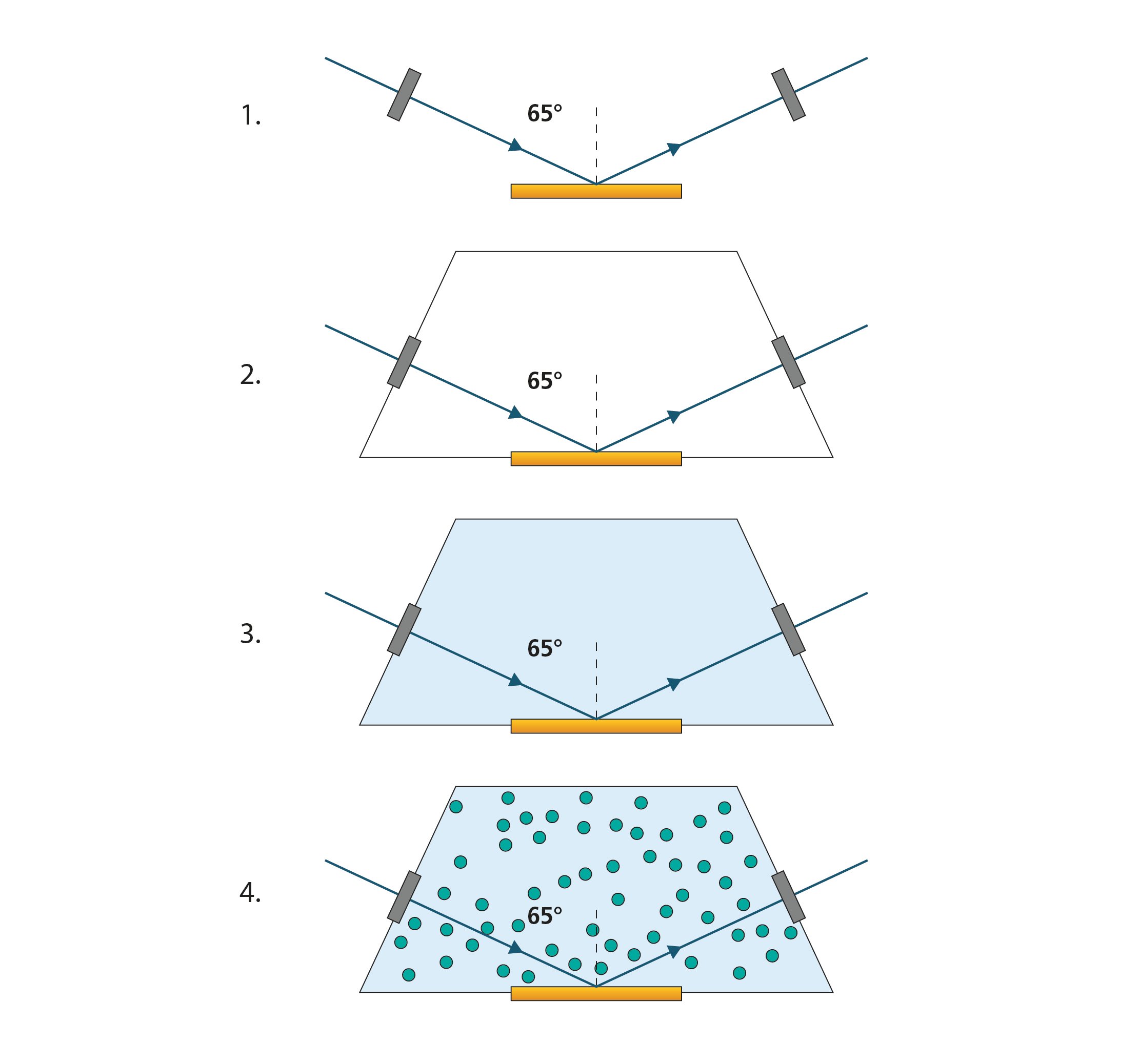
Figure 1. A schematic cross-section of a QSense ellipsometry module with a mounted sensor and the optical model setup step by step.
The first step is to take an SE measurement of the substrate, i.e., the metal-coated QSensor. We should consider the following questions about the substrate so that a well-fitting model can be prepared:
In this example we use gold. In the visible spectrum, gold is absorbing. Because the gold layer is sufficiently thick, the reflected light is sensitive neither to the underlying adhesion layer between the gold and the quartz nor the quartz. Thus, the gold can be considered as a semi-infinite substrate. Note that for oxide surfaces, accurate characterization of the oxide layer thickness and optical properties is essential for analyzing the in-situ experiment.
When the Ellipsometry Module is loaded with the QSensor and mounted onto the Explorer chamber, the ellipsometry probing light beam is able to travel through the module windows and reach the detector. In practice, it is sometimes necessary to manually adjust the angle of incidence (AOI) to perfectly realign the beam with the detector. The module windows may not have been perfectly aligned against the beam due to how they are mounted via O-rings. Changing the AOI from its idealized set point of 65 degrees must be compensated for as a modeled effect on Ψ and Δ. Additionally, the windows, themselves, have an effect on the ellipsometry spectra. Window and AOI offsets are used as fit parameters in the optical model and should be determined via the capturing of a second SE spectrum before proceeding. Typically, the window effects will only modulate Δ and so are parameterized as Δ offsets.
Once the two pre-experiment Ψ and Δ spectra have been captured, the next step is to introduce the solvent that will be used as background solution. In our example, we use buffer solution. Now, the optical model must be adjusted for the change. The ambient material in the model is hence changed from air (or void) to the liquid ambient buffer. The optical properties of the liquid must be known a priori, and may be measured, for example, by the beam deviation method [1]. A colored liquid, with metallic ions, for example, will have non-zero k at wavelengths where light is being absorbed. Ellipsometry data at these wavelengths will commonly be much noisier than for a transparent region.
A third SE measurement is taken to ensure that the adjusted optical model describes the experimental system. Discrepancies between the experimental and model-calculated data may be caused by the rinsing off or attachment of contaminants and for our purposes may be considered by the optical model as substrate modification. The substrate optical properties should be refit at this step.
We now assume that there is a good match between the model-calculated and experimental SE data sets. From this point, differences between the data sets may be attributable to the introduction of the protein solution and the formation of the adsorbate layer. If necessary, the optical properties of the protein solution can be used for the liquid ambient in the optical model during protein solution exposure. Otherwise, we solely attribute modulation of the Ψ and Δ spectra to formation of the adsorbate protein layer.
Now, we are ready to begin the measurement of protein adsorption onto the Au. In the optical model, add an adsorbate layer above the substrate and allow the model to vary the optical properties and/or the thickness of the layer during the experiment. The initial guess value for the thickness of a protein layer can usually be allowed to be 0 nm. As already mentioned, the choice of optical model for the adsorbate layer depends on the expected properties of the layer. In this example, we are adsorbing protein to Au, and will use the de Feijter model. Modern ellipsometry software packages support “dynamic measurements” where ellipsometry spectra are periodically, automatically measured.
During signal baseline stabilization with the background liquid, prior to protein introduction, create a time stamp in QSoft and record the current measurement time for the dynamic ellipsometry measurement. This can be used to synchronize the data for calculating the adsorbate fraction parameters later.
After the experiment has ended, remodeling the ellipsometry data is generally possible if one wishes to try an alternate approach. QCM-D data is also analyzed at this point. Adsorbate thickness or mass versus time data from both instruments may then be exported to obtain the adsorbate fraction parameters versus time.
The ellipsometry and QCM-D measurement start times may be slightly different. To solve this issue, use the time stamp taken by QSoft to synchronize the data so that time t = 0 is the same for both data sets.
Download the white paper to read more about the theory behind the data quantification and the step-by-step procedure on how to do the combined QCM-D and Ellipsometry data analysis.

Malin graduated in engineering physics in 2006, where her research focused on the QCM-D technology. Since then, she has been scrutinizing the how’s and why’s of the world in general, and the world of QCM-D in particular.