Two common types of QCM:s are QCM-D and QCM-I. In this post, we discuss the technical principles behind the two abbreviations, as well as the pros, and cons of the respective method, and when to choose which type.
To get the most out of your QCM measurement and to be able to characterize viscoelastic materials, it is good to collect information about the energy losses, the so-called dissipation or damping. The energy loss can be measured in three different ways, via 1) the resistance, via 2) impedance spectroscopy, and via 3) the decay time of the oscillation. The latter two methods can collect enough information to enable viscoelastic modelling of the QCM data. Below we take a closer look at how the two methods work and how they relate to QCM-I and QCM-D.
QCM-D is short for Quartz Crystal microbalance with Dissipation monitoring and QCM-I is short for Quartz Crystal Microbalance with Impedance spectroscopy. To complicate things a bit however, there are different types of QCM-D:s and there are multiple versions of QCM with impedance spectroscopy. I.e., not all QCM-D:s are based on the same technological principle, and QCM-I is not the only QCM based on impedance spectroscopy. As we mentioned above, the dissipation can be obtained in different ways, for example via the bandwidth, which is an impedance measurement, or via the decay time, also called pinging. Currently, there are QCM-Ds based on both the impedance approach and on pinging. Even if the technological principles of the QCM-D:s in the market differ, they all collect information about the energy losses of the system under study.
In addition to QCM-I, QCM:s with impedance spectroscopy can also be called for example QCM-Z and, as mentioned above, QCM-D. Since the abbreviation doesn’t reveal the technological principle on which the QCM is based, it can be helpful to learn more about the QCM that you are using or planning to purchase as this will give you better insight into the data and how to make the most of it.
To compare the two approaches of measuring the energy loss, via impedance spectroscopy and via pinging, we start by looking at the electrical representation of a quartz crystal, Fig. 1. The equivalent circuit, a so-called Butterworth- Van-Dyke element, consists of a capacitance (C1), inductance (L1), and resistance, (R1), in parallel with a shunt capacitance (C0). In brief, L1 represents the oscillating mass and C1 represents the elasticity of the mass. The resistance, R1, represents the losses in the system, and C0 the electrical component due to the overlap of the electrodes on the crystal.

Figure 1. Representations of A) a quartz crystal and an B) equivalent circuit
With the electrical representation of a quartz crystal, the dissipation is defined according to Eq. 1. I.e., if R1 and L1 are known, the dissipation can be calculated.

As already mentioned, one way to assess the D value is to use impedance (or admittance) spectroscopy, which makes it possible to determine all the elements of the equivalent circuit, Fig. 1.1-3 In an impedance spectroscopy set-up, a sinusoidal voltage, V, is applied over the crystal and the input frequency is varied in a stepwise manner in the frequency range spanning the resonance peak, Fig. 2.
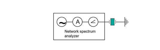
Figure 2. A schematic illustration of QCM with impedance spectroscopy.
At each frequency, the current and phase are recorded. The ratio of the voltage and current gives the frequency dependent impedance, Z, Eqs. 2-4 (or the admittance, Y, which is the reciprocal of the impedance). The impedance of the equivalent circuit can be expressed as
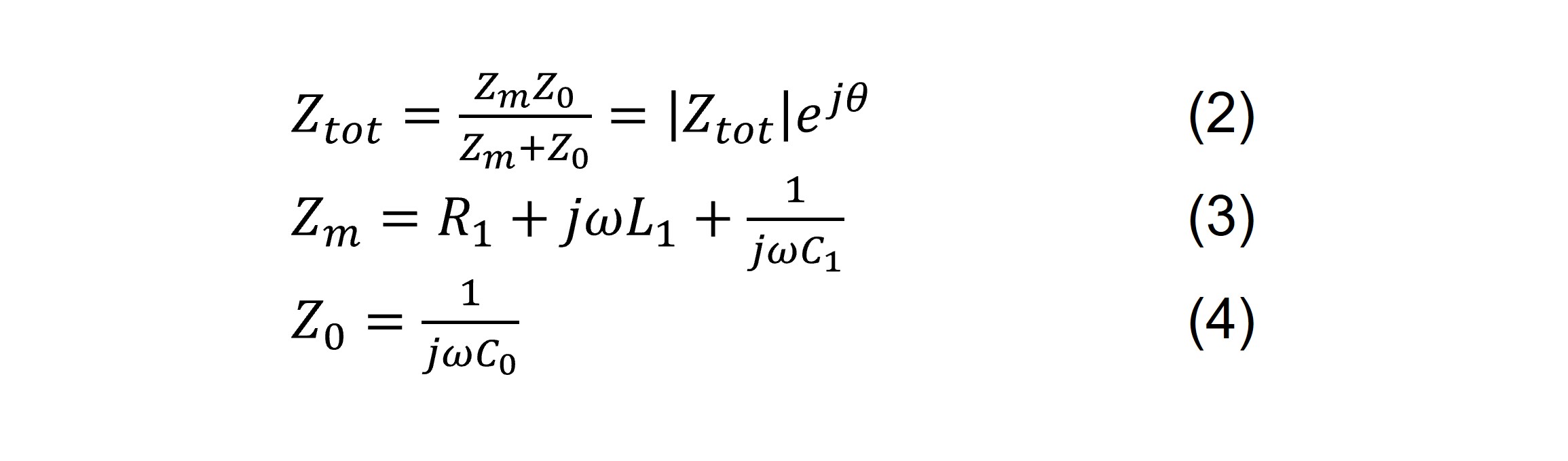
where |Ztot| is the amplitude, θ is the phase angle, and ω=2πf.
When a complete sweep over the frequency range has been recorded, the four parameters C1, L1, R1 and C0 of the electrical equivalent circuit can be fitted numerically. This result can then be used to quantify the parameters of the electrical equivalent circuit, of which L1 and R1 are needed to calculate D according to Eq. 1.
The dissipation, D, can also be obtained by measuring the bandwidth, BW, or half bandwidth at half maximum, Γ, of the resonance peak, and then using Eq. 5.

The equations used to describe the equivalent circuit are only valid in steady state when all transient processes have stopped. Hence, the frequency sweep must be made slow enough to let the crystal stabilize its oscillation at every new frequency step. This fact inflicts a speed limit on the acquisition rate, which makes impedance spectroscopy considerably slower than for example QCM and QCM-R.4 However the full characterization of the equivalent circuit enables the extraction of the dissipation in the system, not only a relative measure as with resistance measurements.
The decay-based approach, also referred to as ‘pinging’ was developed by Rodahl et al. in the 90s.5 This technical solution was the origin of QSense QCM-D and is still the technical principle on which all QSense instruments are based.
With the pinging method, the QCM crystal is rapidly excited to resonance, the driving voltage is turned off, and then the decay time of the oscillation is monitored. The decay is then numerically fitted to an exponentially damped sinusoidal and D can then be extracted along with the resonant frequency of the sensor. This measurement is very fast, and the high acquisition rate makes it is possible to record several harmonics with good data quality, which in turn enables high-resolution kinetic studies and viscoelastic modeling.5
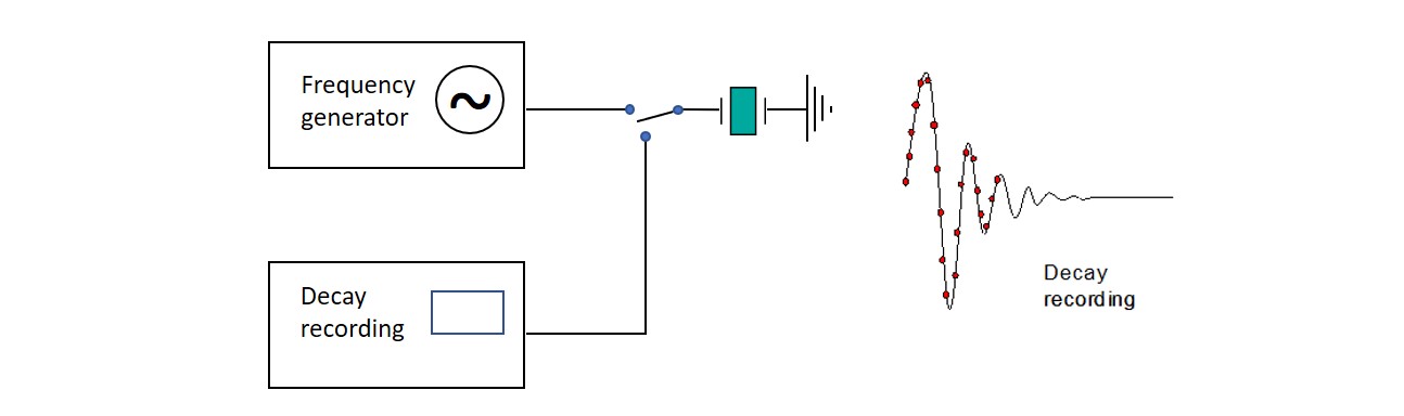 Figure 3. Principle of decay-based Dissipation monitoring. The crystal is exited into oscillation during a short time, after which the driving frequency is switched off, and the freely oscillating decay is recorded. Since only one decay recording is necessary to determine both frequency and dissipation, the acquisition is very fast.
As all methods, both the impedance approach and the decay time measurement have their pros and cons. A strength of both approaches is that, compared to for example QCM and QCM-R, QCM measurements with impedance and QCM with decay time measurement contain enough information to extract the D-value. Both methods also allow for overtone measurements. As these are two prerequisites for viscoelastic modelling, both methods allow for such quantification.
A drawback with impedance measurements is that it can be slow. The frequency sweeps are lengthy, which makes the measurements slow and limits the maximum time resolution. Also, the measurement is sensitive to small variations in the shunt capacitance, C0, which can influence the accuracy and/or noise of the measurement.
The decay based QCM doesn’t really have any technical drawbacks. Unlike the impedance approach, the pinging principle is very fast, which enables a high time resolution. Also, the decay approach doesn’t experience the same sensitivity to variations in the shunt capacitance since the short circuit mode practically eliminates the interference from the shunt and stray capacitance. This makes the method very stable. A drawback relative to the impedance approach worth mentioning however, is the cost of the instruments. Decay based QCM:s tend to be more expensive than impedance based ones.
The pros and cons of the two types of QCM:s make them suitable for different kinds of applications. Note that even if QCM-I and QCM-D output different parameters, you can still extract the exact same information regarding the film, using the equations above. Table 1 summarizes some of the key aspects and exemplifies when to use which method.
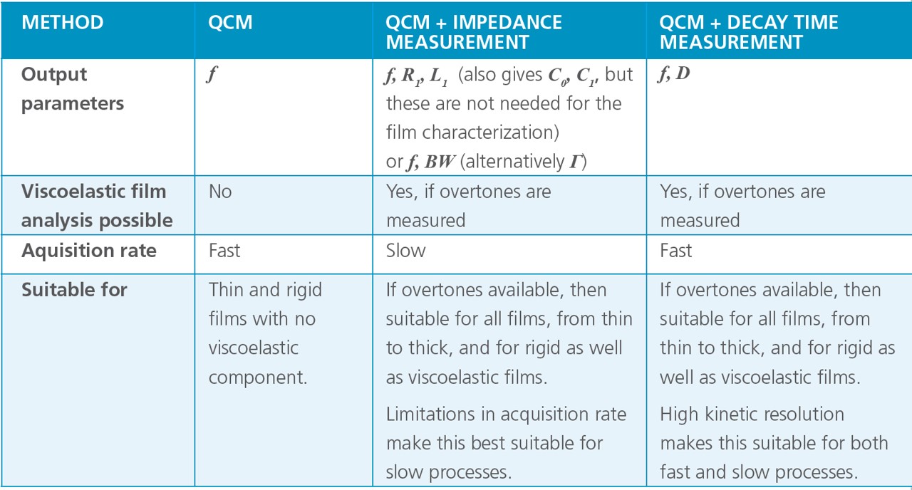
Table 1. Comparison of QCM, QCM with impedance and QCM with decay measurement.
QCM-D and QCM-I are two common QCM:s that can be based on either impedance measurement or decay time measurement, so-called pinging. The first QCM-D in the market was based on the pinging approach which was developed by Rodahl et al in the 90’s. Since then, QCM-D:s based on the impedance approach have also appeared. In generals, both technical solutions allow for collection of enough information, i.e., f and D at multiple harmonics, to enable viscoelastic modelling.


Fredrik is a Senior Application Scientist at Biolin Scientific. After his Master of Science in Biosensors- and Microsystems technology he has worked with technology and application development in as diverse fields as electroporation, multivariate gas sensing, drug screening and surface science.