Advanced QCMs like QCM-D, QCM-A, and QCM-I all give you information on energy loss in the system that you are studying. But there are different ways to measure these losses, and not all QCMs do it the same way. Here, we will break down the different methods and their pros and cons to help you understand these differences so that you will be better equipped to choose the right QCM for your needs and ensure accurate and reliable measurements.
As discussed in previously published posts, the dissipation contains information about the material under study. This is particularly apparent when you use QCM to study viscoelastic layers, where the wave propagation is very different from that of quartz. The energy losses in such films can be significant and information about the dissipation is therefore very valuable, and even critical, not only to determine what approach to use for the mass and thickness quantifications but also to be used as input for viscoelastic analysis and modeling, when applicable.1
There are three main ways to extract information about the energy loss, the D-value, in the system that is being studied. The three ways are:
One way to assess the D-value is to use impedance or admittance spectroscopy.2,3 Here, a sinusoidal voltage, V, is applied over the crystal and the resulting current, I, is measured as a function of the frequency of the applied voltage. The ratio of the voltage and current will then give the frequency-dependent impedance, Z. The admittance, Y, which is the reciprocal of the impedance, can also be extracted. This result can then be used to quantify the parameters of the electrical equivalent circuit, Fig. 1A, of which L1 and R1 are needed to calculate D.
The D value can also be obtained by measuring the bandwidth, or half bandwidth at half maximum, Γ, of the resonance peak, Fig. 1B, and then using Eq. 1.

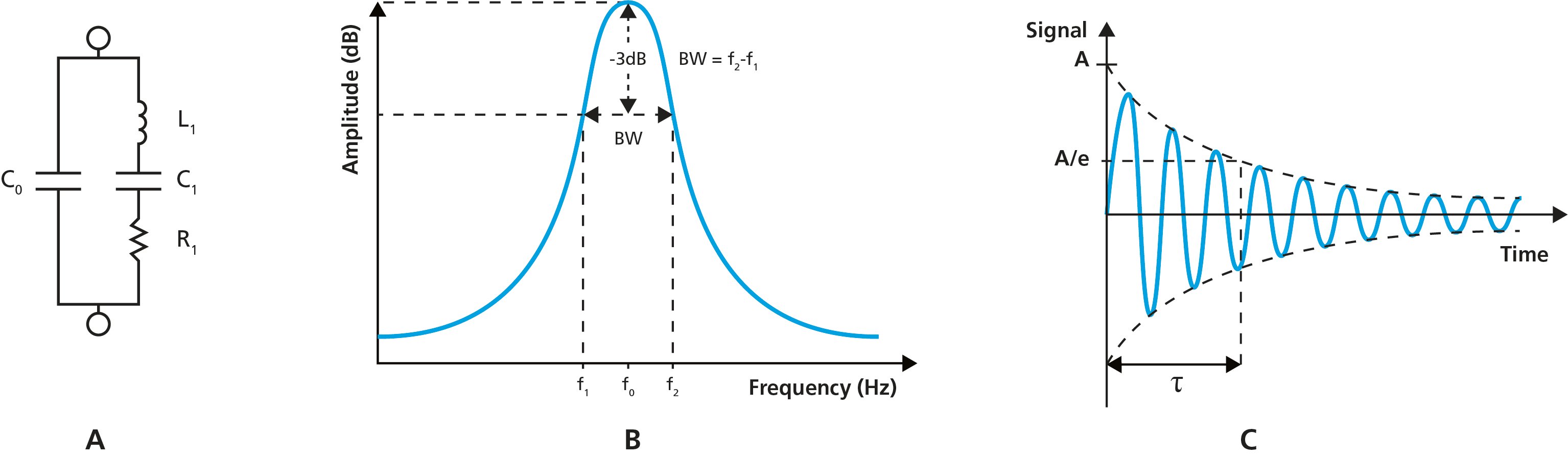
Figure 1. A) Equivalent circuit of a quartz crystal sandwiched between two electrodes, the motional arm being the branch to the right. B) schematic illustration of the resonance peak, showing the center frequency, f0, and the bandwidth, BW, which gives the D-value. C) A damped oscillation with maximum amplitude A and decay time τ.
Another approach to extract the D is to measure the decay time, τ, of the crystal oscillation, Fig. 1C, and use Eq. 2.4,5 In this so-called pinging approach, the crystal is rapidly excited to resonance, the driving voltage is then turned off and the decay time of the oscillation is monitored. D can then be extracted along with the resonant frequency of the sensor.

The resistance, R, is essentially equivalent to the resistor in the motional arm in the circuit in Fig. 1A and can be measured, for example, via an advanced oscillator circuit.6
Each of these methods, to measure the energy losses in the system and to get the D-value - impedance-, pinging-, and resistance measurement, is associated with some pros and cons such as time resolution and information content.
A benefit of impedance measurements is that they contain enough information to extract the D value, and it is also possible to measure several harmonics of the crystal oscillator. These are two prerequisites for viscoelastic modeling.
A drawback of this method is that the frequency sweeps are lengthy, which makes the measurements slow and limits the maximum time resolution. Another drawback is that the measurement is sensitive to small variations in the shunt capacitance, which can influence the accuracy and/or noise of the measurement.
There are several benefits to this method. As with the impedance frequency sweep method, pinging allows for overtone measurements which makes viscoelastic modelling possible. The pinging principle is also very fast, which enables a high time resolution. Additionally, the short circuit mode practically eliminates the interference from the shunt and stray capacitance, which greatly improves measurement stability.
The R parameter alone cannot be used to calculate the D value. Also, when letting the QCM sensor be a part of an oscillator circuit, only one resonance frequency is measured. Hence, this method does not allow for viscoelastic modeling and R can only be used as an indicator of the energy losses in the system. The oscillator circuits are generally sensitive to changes in stray capacitance, making it hard to obtain a stable measurement.
In conclusion, understanding the energy loss in a system using QCM measurements is crucial, particularly for analyzing viscoelastic layers. Advanced QCMs like QCM-D, QCM-A, and QCM-I offer different methods to measure dissipation, using impedance spectroscopy, decay time measurement, or resistance measurements. Each method has its advantages and drawbacks.
Download the overview to learn more about dissipation and why it matters in QCM measurements


Malin graduated in engineering physics in 2006, where her research focused on the QCM-D technology. Since then, she has been scrutinizing the how’s and why’s of the world in general, and the world of QCM-D in particular.

