In QCM-D measurements, the D-factor provides information that is complementary to the frequency response, but how can this information be understood? In this post, we dig a bit deeper into the behavior of the sensor oscillation at various types of loads and take a closer look at what the D-factor reveals.
When a resonator is loaded with a thin and rigid film, the resonance frequency will decrease as an indication of increased mass. If the film is much thinner than the thickness of the resonator, the decrease in resonance frequency (f) is linearly correlated to the increase in mass (m) (or thickness) according to the Sauerbrey relation:

where the constant C is material characteristic and n is the overtone number, n = 1 denoting the fundamental frequency. For a quartz crystal with a fundamental frequency of 5 MHz, the constant C is 17.7 ng/(cm2∙Hz).
A thin, rigid film is purely elastic, just as the quartz crystal itself. If a viscous component is introduced as well, thus giving a viscoelastic or soft film, there will be energy losses in the system. Let’s now consider a soft film adsorbed on a quartz sensor oscillating in bulk water, such as a hydrated polymer material. In Fig. 1 A-B, the responses of the resonance frequency, f, and energy dissipation factor, D, are shown as a function of film thickness. For very thin films (a few nanometers) both the f and D responses are small and change in a linear fashion. This indicates that the Sauerbrey equation, eq. 1, still gives an adequate description of the system. As the thickness increases, Fig. 1 A-B, the change in f and D enter a non-linear regime and the D response becomes considerable.
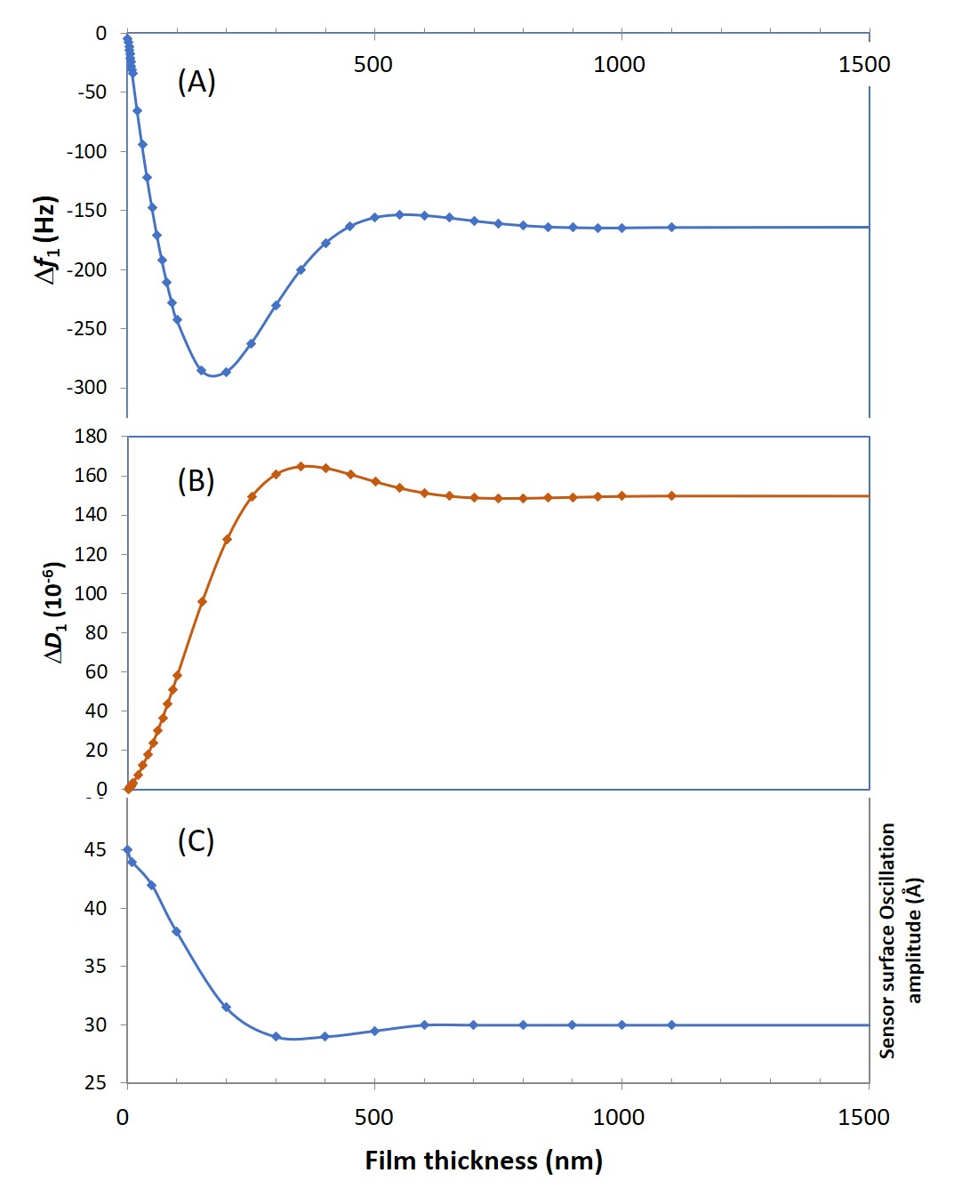
Figure 1. Simulated QCM-D responses, as a function of film thickness, for the first harmonic, n = 1. In (A) the frequency response, f, and in (B) the dissipation factor, D. (C) shows how the sensor maximum oscillation amplitude varies as a function of the thickness of the added layer.
In the case of a rigid film, it will couple perfectly to the oscillating motion of the sensor surface. A soft film, on the other hand, will have a delayed motion as the viscoelastic shear wave introduced by the oscillation propagates through the film. This propagation of the shear wave, and the softness of the film, will have a dampening effect on the oscillating motion, which is quantified through the dissipation factor, D.

Due to reflection of the acoustic wave at the film-liquid interface, there could be positive or negative superposition between impinging and reflecting waves. This can be seen in Fig. 1C, where the sensor oscillation amplitude as a function of film thickness is plotted.
At a distance coinciding with the peak in D, the oscillation amplitude of the sensor surface goes from decreasing to increasing trend. The result is that the resistance to motion that is experienced by the sensor surface can either be amplified or reduced, depending on the superposition of the acoustic waves. Less shear resistance will result in larger oscillation amplitude and lower energy dissipation factor. A negative shear resistance effect will at the same time have a relieving effect on the resonance frequency since the experienced mass load is decreased. This can be seen for thicknesses between 150 and 500 nm for f, Fig 1A, and 350 and 650 nm for D, Fig 1B, in this example.
It should be noted that the minimum point for f, Fig 1A, coincides with the maximum slope for D, Fig 1B, and that the maximum point for D coincides with the maximum upwards slope for f. The latter point corresponds to the case of having maximum antiphase between the impinging and reflected acoustic shear wave, giving maximum energy losses and thus maximum D. At the former point, the experienced mass is at maximum and the derivative of the energy losses is at maximum.
Thus, it is clear that the shapes of f and D will describe the situation in different ways in the viscoelastic regime. When plotting Δf versus ΔD, Fig. 2, this becomes even clearer that at some point it is not possible to draw the correct conclusions from f only. If one for example consider the case of having a ΔD of 149∙10-6, this corresponds to three different Df values -155, -161 and -263 Hz.
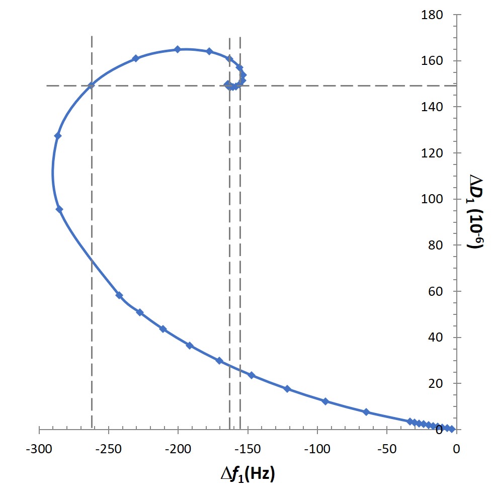
Figure 2. Simulated QCM-D responses, as a function of film thickness, for the first harmonic, n = 1, plotted as Δf versus ΔD. The graph shows that for viscoelastic layers, the f:s and D:s could be non-unique. For example, in this graph, ΔD = 149∙10-6 corresponds to three different Df values -155, -161 and -263 Hz.
Want to save the text for later? Download the text as pdf below

Gabriel Ohlsson, Ph.D., is a former employee at Biolin Scientific where he initially held a position as an application scientist and later as a sales manager. Dr. Ohlsson did his Ph.D. in engineering physics and has spent a lot of time developing sensing technologies for soft matter material applications. One of his main tools during this research has been the QCM-D technology.